تسارع ظاهرة الاحتباس الحراري بسبب التغذية المرتدة من دورة الكربون في نموذج مناخي مقترن
بيتر م. كوكس ، ريتشارد أ. بيتس ، كريس دي جونز ، ستيفن أ. سبال وإيان جيه توتيرديل

Naturevolume 408 ، الصفحات 184-187 (2000) | تحميل الاقتباس
نُشرت Erratum في هذا المقال في 7 ديسمبر 2000
نبذة مختصرة
من المتوقع أن تؤدي الزيادة المستمرة في تركيز ثاني أكسيد الكربون في الغلاف الجوي نتيجة للانبعاثات البشرية المنشأ إلى تغييرات كبيرة في المناخ 1. يتم امتصاص حوالي نصف الانبعاثات الحالية من قبل المحيطات والنظم الإيكولوجية البرية 2 ، ولكن هذا الامتصاص حساس للمناخ 3.4 وكذلك لتركيزات ثاني أكسيد الكربون في الغلاف الجوي 5 ، مما يخلق حلقة تغذية مرتدة. استبعدت نماذج الدورة العامة عمومًا التغذية المرتدة بين المناخ والغلاف الحيوي ، باستخدام توزيعات الغطاء النباتي الثابتة وتركيزات ثاني أكسيد الكربون من نماذج دورة الكربون البسيطة التي لا تشمل تغير المناخ 6. نقدم هنا نتائج من خلال نموذج ثلاثي الأبعاد وثاني أكسيد الكربون مقترن تمامًا ، مما يشير إلى أن التغذية المرتدة من دورة الكربون يمكن أن تسرع بشكل كبير من تغير المناخ خلال القرن الحادي والعشرين. نجد أنه في إطار سيناريو "العمل كالمعتاد" ، يعمل المحيط الحيوي للأرض كغوص كلي للكربون حتى عام 2050 ، لكنه يتحول إلى مصدر بعد ذلك. بحلول عام 2100 ، يكون معدل امتصاص المحيطات البالغ 5 جيغا طن في السنة متوازنا مع مصدر الكربون الأرضي ، وتركيزات ثاني أكسيد الكربون في الغلاف الجوي تبلغ 250 مساءً. أعلى في محاكاةنا المزدوجة تمامًا مقارنة بنماذج الكربون غير المنفصلة 2 ، مما ينتج عنه ارتفاع في درجة الحرارة على مستوى عالمي يبلغ 5.5 كلفن ، مقارنةً بـ 4 كلفن دون ردود فعل دورة الكربون.
تم توفير الوصول بواسطة بوابة المجلس الرئاسي التخصصي للتعليم والبحث العلمي
الأساسية
يعتمد نموذج الدوران العام (GCM) الذي قمنا باستخدامه على نموذج هادل 37 - المحيط والغلاف الجوي المقترن ، HadCM37 ، والذي قمنا بربطه بنموذج دورة الكربون في المحيط (HadOCC) ونموذج الغطاء النباتي العالمي الديناميكي (TRIFFID). فيزياء الغلاف الجوي وديناميات GCM لدينا مماثلة لتلك المستخدمة في HadCM3 ، ولكن حساب حسابية إضافية بما في ذلك دورة الكربون التفاعلية جعلت من الضروري خفض دقة المحيط إلى 2.5 درجة مئوية و 3.75 درجة ، مما يستلزم استخدام تعديلات التدفق في عنصر المحيط لمواجهة الانجراف المناخ. حسابات HadOCC لتبادل ثاني أكسيد الكربون بين الغلاف الجوي والمحيطات ، ونقل ثاني أكسيد الكربون إلى العمق من خلال كل من مضخة الذوبان والمضخة البيولوجية 8. نموذج TRIFFID حالة المحيط الحيوي من حيث الكربون التربة ، وهيكل وتغطية خمسة أنواع وظيفية من النبات داخل كل نموذج الشبكة (شجرة عريضة الأوراق ، شجرة needleleaf ، العشب C3 ، العشب C4 والشجيرة). مزيد من التفاصيل حول HadOCC و TRIFFID مذكورة في الطرق.
تم إحضار نموذج دورة المناخ / الكربون المقترن بالتوازن مع تركيز ثاني أكسيد الكربون في الغلاف الجوي "قبل الصناعة" بمقدار 290 مساءً ، بدءًا من مجموعة بيانات عن الغطاء الأرضي المرصودة 9. كانت الحالة الناتجة مستقرة ، مع تدفقات ضئيلة من الغلاف الجوي الصافي للأرض والغلاف الجوي والمحيطات في المدى الطويل ، وعدم وجود انحراف ملحوظ في تركيز ثاني أكسيد الكربون في الغلاف الجوي. تنتج هذه المحاكاة مواقع المناطق الأحيائية الرئيسية للأرض ، وتقديرات للكربون المحيطي (38100 جيجا جيم) وكربون النبات (493 جيجا جيم) وكربون التربة (1180 جيجا جيم) والإنتاجية الأولية الصافية للأرض (60 جيجا طن سنويا -1) التي تقع ضمن نطاق التقديرات الأخرى 2،10،11،12. تتوافق الإنتاجية الأولية للمحيطات أيضًا مع النتائج المستمدة من الاستشعار عن بُعد 13 ، 14 ، مما ينتج عنه إجمالي عالمي يبلغ 53 جيجا س س عام -1 ، وتغيرات موسمية وخطية واقعية 15.
تعرض دورة الكربون المحاكاة تباينًا كبيرًا بين الأعوام ، مدفوعًا بظاهرة النينيو / التذبذب الجنوبي (ENSO). تعد الاستجابة الواقعية لتقلب المناخ الداخلي شرطا مسبقا هاما لأي نموذج لدورة الكربون لاستخدامه في التنبؤ بتغير المناخ. ترتبط التقلبات في ثاني أكسيد الكربون في الغلاف الجوي السنوي مع مرحلة ENSO ، كما هو مبين في مؤشر Nino3 (الشكل 1). أثناء ظروف ظاهرة النينيو (إيجابية Nino3) ، يحاكي النموذج زيادة في ثاني أكسيد الكربون في الغلاف الجوي ؛ هذه الزيادة ناتجة عن المحيط الحيوي الأرضي الذي يعمل كمصدر كبير (خاصة في Amazonia16) ، والذي لا يتم تعويضه جزئيًا إلا عن طريق خفض إطلاق الغازات من المحيط الهادي الاستوائي. العكس هو الصحيح خلال مرحلة النينيا. تتوافق الحساسية الكلية لدورة الكربون المصممة لتغير ENSO مع سجل الرصد 17 ، مما يدل على أن النظام المقترن يستجيب بشكل واقعي للتشوهات المناخية.
الشكل 1: التباين النمذجي والملاحظ بين فترات تركيز غاز ثاني أكسيد الكربون في الغلاف الجوي.
شكل 1
يوضح الشكل الشذوذ في معدل نمو ثاني أكسيد الكربون في الغلاف الجوي مقابل مؤشر Nino3 ، المأخوذ من محاكاة التحكم قبل الصناعي (الصلبان) وملاحظات مونا لوا (مثلثات). (مؤشر Nino3 هو متوسط شذوذ درجة حرارة سطح البحر السنوي في المحيط الهادي الاستوائي ، 150 درجة مئوية - 90 درجة غربا ، 5 درجة جنوبا - 5 درجة شمالا). تمثل تدرجات الخطوط المتقطعة والمتقطعة حساسية t
Acceleration of global warming due to carbon-cycle feedbacks in a coupled climate model
Nature
408,
184–187 (2000)
Abstract
The continued increase in the atmospheric concentration of carbon dioxide due to anthropogenic emissions is predicted to lead to significant changes in climate1. About half of the current emissions are being absorbed by the ocean and by land ecosystems2, but this absorption is sensitive to climate3,4 as well as to atmospheric carbon dioxide concentrations5, creating a feedback loop. General circulation models have generally excluded the feedback between climate and the biosphere, using static vegetation distributions and CO2 concentrations from simple carbon-cycle models that do not include climate change6. Here we present results from a fully coupled, three-dimensional carbon–climate model, indicating that carbon-cycle feedbacks could significantly accelerate climate change over the twenty-first century. We find that under a ‘business as usual’ scenario, the terrestrial biosphere acts as an overall carbon sink until about 2050, but turns into a source thereafter. By 2100, the ocean uptake rate of 5 Gt C yr-1 is balanced by the terrestrial carbon source, and atmospheric CO2 concentrations are 250 p.p.m.v. higher in our fully coupled simulation than in uncoupled carbon models2, resulting in a global-mean warming of 5.5 K, as compared to 4 K without the carbon-cycle feedback.
Access provided by Specialized Presidential Council for Educ and Scientific Research Portal
Main
The general circulation model (GCM) that we used is based on the third Hadley Centre coupled ocean–atmosphere model, HadCM37, which we have coupled to an ocean carbon-cycle model (HadOCC) and a dynamic global vegetation model (TRIFFID). The atmospheric physics and dynamics of our GCM are identical to those used in HadCM3, but the additional computational expense of including an interactive carbon cycle made it necessary to reduce the ocean resolution to 2.5° × 3.75°, necessitating the use of flux adjustments in the ocean component to counteract climate drift. HadOCC accounts for the atmosphere–ocean exchange of CO2, and the transfer of CO2 to depth through both the solubility pump and the biological pump8. TRIFFID models the state of the biosphere in terms of the soil carbon, and the structure and coverage of five functional types of plant within each model gridbox (broadleaf tree, needleleaf tree, C3 grass, C4 grass and shrub). Further details on HadOCC and TRIFFID are given in Methods.
The coupled climate/carbon-cycle model was brought to equilibrium with a ‘pre-industrial’ atmospheric CO2 concentration of 290 p.p.m.v., starting from an observed landcover data set9. The resulting state was stable, with negligible net land–atmosphere and ocean–atmosphere carbon fluxes in the long-term mean, and no discernible drift in atmospheric CO2 concentration. This simulation produces the locations of the main land biomes, and estimates of ocean carbon (38,100 Gt C), vegetation carbon (493 Gt C), soil carbon (1,180 Gt C) and terrestrial net primary productivity (60 Gt C yr-1) that are within the range of other estimates2,10,11,12. Ocean primary productivity is also compatible with results derived from remote sensing13,14, producing a global-mean total of 53 Gt C yr-1, and realistic seasonal and latitudinal variations15.
The simulated carbon cycle displays significant interannual variability, which is driven by the model-generated El Niño/Southern Oscillation (ENSO). A realistic response to internal climate variability is an important prerequisite for any carbon-cycle model to be used in climate change predictions. Fluctuations in annual-mean atmospheric CO2 are correlated with the phase of ENSO, as indicated by the Nino3 index (Fig. 1). During El Niño conditions (positive Nino3), the model simulates an increase in atmospheric CO2; this increase results from the terrestrial biosphere acting as a large source (especially in Amazonia16), which is only partially offset by a reduced outgassing from the tropical Pacific Ocean. The opposite is true during the La Niña phase. The overall sensitivity of the modelled carbon cycle to ENSO variability is consistent with the observational record17, demonstrating that the coupled system responds realistically to climate anomalies.
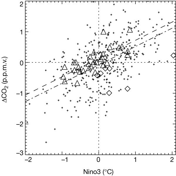
The figure shows the anomaly in the growth rate of atmospheric CO2 versus the Nino3 index, taken from our pre-industrial control simulation (crosses) and the Mauna Loa observations (triangles). (The Nino3 index is the annual mean sea surface temperature anomaly in the tropical Pacific, 150° W–90° W, 5° S–5° N.) The gradients of the dashed and dot-dashed lines represent the sensitivity of the carbon cycle to ENSO, as given by the observations and the model, respectively. We have excluded observations that immediately follow major volcanic events (data points shown by diamonds), since during these years the carbon cycle may have been significantly perturbed by the induced tropospheric cooling.
Transient simulations were carried out for 1860–2100, using CO2emissions as given by the IS92a scenario18. Other greenhouse gases were also prescribed from IS92a, but the radiative effects of sulphate aerosols were omitted. Three separate runs were completed to isolate the effect of climate/carbon-cycle feedbacks; an experiment with prescribed IS92a CO2 and fixed vegetation (that is, a ‘standard’ GCM climate change simulation), an experiment with interactive CO2 and dynamic vegetation but no direct effects of CO2 on climate (akin to ‘offline’ carbon-cycle projections that neglect climate change6), and a fully coupled climate/carbon-cycle simulation.
Figure 2 shows results from the fully coupled run. From 1860 to 2000, the simulated stores of carbon in the ocean and on land increase by about 100 Gt C and 75 Gt C, respectively. However, the atmospheric CO2 is 15–20 p.p.m.v. too high by the present day (corresponding to a timing error of about 10 years). Possible reasons for this include an overestimate of the prescribed net land-use emissions and the absence of other important climate forcing factors. The modelled global mean temperature increase from 1860 to 2000 is about 1.4 K (Fig. 3b), which is higher than observed19, probably due to the absence of cooling from anthropogenic aerosols20. Offline tests suggest that such a relative warming can suppress the terrestrial carbon sink by enhancing soil and plant respiration11. Nevertheless, the rate of increase of CO2 from 1950 to 2000 closely follows the recent observational record, which implies that the airborne fraction is being well simulated over this period. For the 20 years centred on 1985, the mean land and ocean uptake of carbon are 1.5 and 1.6 Gt yr-1, respectively (compare best estimates for the 1980s of 1.8 ± 1.8 and 2.0 ± 0.8 Gt yr-1)2. The model therefore captures the most important characteristics of the present-day carbon cycle.
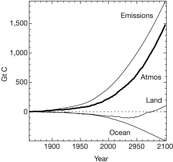
The thick line shows the simulated change in atmospheric CO2. The thinner lines show the integrated impact of the emissions, and of land and ocean fluxes, on the atmospheric CO2increase, with negative values implying net uptake of CO2. We note that the terrestrial biosphere takes up CO2 at a decreasing rate from about 2010 onwards, becoming a net source at around 2050. By 2100 this source from the land almost balances the oceanic sink, so that atmospheric carbon content is increasing at about the same rate as the integrated emissions (that is, the airborne fraction is ∼1).
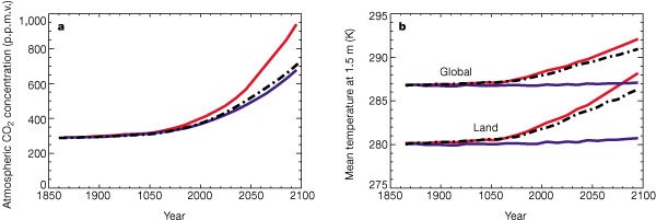
a, Global-mean CO2 concentration, and b, global-mean and land-mean temperature, versus year. Three simulations are shown; the fully coupled simulation with interactive CO2 and dynamic vegetation (red lines), a standard GCM climate change simulation with prescribed (IS92a) CO2 concentration and fixed vegetation (dot-dashed lines), and the simulation which neglects direct CO2-induced climate change (blue lines). The slight warming in the latter is due to CO2-induced changes in stomatal conductance and vegetation distribution.
The simulated atmospheric CO2 diverges much more rapidly from the standard IS92a concentration scenario in the future. First, vegetation carbon in South America begins to decline, as a drying and warming of Amazonia initiates loss of forest (Fig. 4a). This is driven purely by climate change, as can be seen by comparing the fully coupled run (red lines) to the run without global warming (blue lines). The effects of anthropogenic deforestation on landcover are neglected in both cases. A second critical point is reached at about 2050, when the land biosphere as a whole switches from being a weak sink for CO2 to being a strong source (Fig. 2). The reduction in terrestrial carbon from around 2050 onward is associated with a widespread climate-driven loss of soil carbon (Fig. 4b). An increase in the concentration of atmospheric CO2 alone tends to increase the rate of photosynthesis and thus terrestrial carbon storage, provided that other resources are not limiting4. However, plant maintenance and soil respiration rates both increase with temperature. As a consequence, climate warming (the indirect effect of a CO2 increase) tends to reduce terrestrial carbon storage11, especially in the warmer regions where an increase in temperature is not beneficial for photosynthesis. At low CO2 concentrations the direct effect of CO2dominates, and both vegetation and soil carbon increase with atmospheric CO2. But as CO2 increases further, terrestrial carbon begins to decrease, because the direct effect of CO2 on photosynthesis saturates but the specific soil respiration rate continues to increase with temperature. The transition between these two regimes occurs abruptly at around 2050 in this experiment ( Fig. 4b). The carbon stored on land decreases by about 170 Gt C from 2000 to 2100, accelerating the rate of atmospheric CO2 increase over this period.
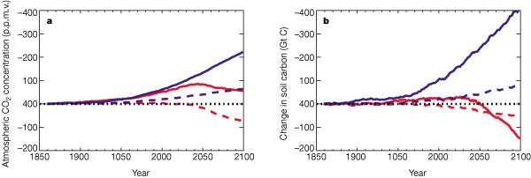
The red lines represent the fully coupled climate/carbon-cycle simulation, and the blue lines are from the ‘offline’ simulation which neglects direct CO2-induced climate change. The figure shows simulated changes in vegetation carbon (a) and soil carbon (b) for the global land area (continuous lines) and South America alone (dashed lines).
The ocean takes up about 400 Gt C over the same period, but at a rate which is asymptotically approaching 5 Gt C yr-1 by 2100. This reduced efficiency of oceanic uptake is partly a consequence of the nonlinear dependence of the partial pressure of dissolved CO2 on the total ocean carbon concentration, but may also have contributions from climate change3. Although the thermohaline circulation of the ocean weakens21by about 25% from 2000 to 2100, this is much less of a reduction than seen in some previous simulations22, and the corresponding effect on ocean carbon uptake is less significant. In our experiment, increased thermal stratification due to warming of the sea surface suppresses upwelling, which reduces nutrient availability and lowers primary production by about 5%. However, ocean-only tests suggest a small effect of climate change on oceanic carbon uptake, as this reduction in the biological pump is compensated by reduced upwelling of deep waters which have high concentrations of total carbon.
By 2100 the modelled CO2 concentration is about 980 p.p.m.v. in the coupled experiment, which is more than 250 p.p.m.v. higher than the standard IS92a scenario or that simulated in the ‘offline’ experiment (Fig. 3a). As a result, the global-mean land temperatures increase from 1860 to 2100 by about 8 K, rather than the 5.5 K of the standard scenario (Fig. 3b).
These numerical experiments demonstrate the potential importance of climate/carbon-cycle feedbacks, but the magnitude of these in the real Earth system is still highly uncertain. Terrestrial carbon models differ in their responses to climate change11,12, owing to gaps in basic understanding of processes. For example, the potential conversion of the global terrestrial carbon sink to a source is critically dependent upon the long-term sensitivity of soil respiration to global warming, which is still a subject of debate23. The experiments presented here exclude the potentially large direct human influences on terrestrial carbon uptake through changes in landcover and land management. Local effects, such as the possible climate-driven loss of the Amazon rainforest, rest upon uncertain aspects of regional climate change, and may be ‘short-circuited’ by direct human deforestation. A full assessment of the uncertainties must await further coupled experiments utilizing alternative representations of processes and including a more complete set of natural and anthropogenic forcing factors (for example, land-use change, forest fires, sulphate aerosol concentrations and nitrogen deposition). However, our results indicate that it will be essential to accurately represent previously neglected carbon-cycle feedbacks if we are to successfully predict climate change over the next 100 years.
Methods
Ocean carbon-cycle model
The inorganic component of HadOCC has been extensively tested as part of the Ocean Carbon Cycle Intercomparison Project; it was found to reproduce tracer distributions to an accuracy consistent with other ocean GCMs24. The biological component treats four additional ocean fields: nutrient, phytoplankton, zooplankton and detritus8. The phytoplankton population changes as a result of the balance between growth, which is controlled by light level and the local concentration of nutrient, and mortality, which is mostly as a result of grazing by zooplankton. Detritus, which is formed by zooplankton excretion and by phyto- and zooplankton mortality, sinks at a fixed rate and slowly remineralizes to reform nutrient and dissolved inorganic carbon. Thus both nutrient and carbon are absorbed by phytoplankton near the ocean surface, pass up the food chain to zooplankton, and are eventually remineralized from detritus in the deeper ocean. The model also includes the formation of calcium carbonate and its dissolution at depth (below the lysocline).
Terrestrial carbon-cycle model
TRIFFID (top-down representation of interactive foliage and flora including dynamics) has been used offline in a comparison of dynamic global vegetation models11. Carbon fluxes for each vegetation type are calculated every 30 minutes as a function of climate and atmospheric CO2 concentration, from a coupled photosynthesis/stomatal-conductance scheme25,26, which utilizes existing models of leaf-level photosynthesis in C3 and C4 plants27,28. The accumulated fluxes are used to update the vegetation and soil carbon every 10 days. The natural landcover evolves dynamically based on competition between the vegetation types, which is modelled using a Lotka–Volterra approach and a tree–shrub–grass dominance hierarchy. We also prescribe some agricultural regions, in which grasslands are assumed to be dominant. Carbon lost from the vegetation as a result of local litterfall or large-scale disturbance is transferred into a soil carbon pool, where it is broken down by microorganisms that return CO2 to the atmosphere. The soil respiration rate is assumed to double for every 10 K of warming29, and is also dependent on the soil moisture content30. Changes in the biophysical properties of the land surface5, as well as changes in terrestrial carbon, feed back onto the atmosphere.
References
- 1Houghton, J. T. et al. (eds) Climate Change 1995: The Science of Climate Change (Cambridge Univ. Press, Cambridge, 1996).
- 2Schimel, D. et al. in Climate Change 1995: The Science of Climate Change Ch. 2 (eds Houghton, J. T. et al.) 65–131 (Cambridge Univ. Press, Cambridge, 1995).
- 3Sarmiento, J., Hughes, T., Stouffer, R. & Manabe, S. Simulated response of the ocean carbon cycle to anthropogenic climate warming. Nature393, 245–249 ( 1998).
- 4Cao, M. & Woodward, F. I. Dynamic responses of terrestrial ecosystem carbon cycling to global climate change. Nature 393, 249–252 (1998).
- 5Betts, R. A., Cox, P. M., Lee, S. E. & Woodward, F. I. Contrasting physiological and structural vegetation feedbacks in climate change simulations. Nature 387, 796–799 (1997).
- 6Enting, I., Wigley, T. & Heimann, M. Future Emissions and Concentrations of Carbon Dioxide; Key Ocean/Atmosphere/Land Analyses (Technical Paper 31, Division of Atmospheric Research, CSIRO, Melbourne, 1994).
- 7Gordon, C. et al. The simulation of SST, sea ice extents and ocean heat transports in a version of the Hadley Centre coupled model without flux adjustments. Clim. Dyn. 16, 147–168 (2000).
- 8Palmer, J. R. & Totterdell, I. J. Production and export in a global ocean ecosystem model. Deep-Sea Res. (in the press).
- 9Wilson, M. F. & Henderson-Sellers, A. A global archive of land cover and soils data for use in general circulation climate models. J. Clim. 5, 119–143 ( 1985).
- 10Zinke, P. J., Stangenberger, A. G., Post, W. M., Emanuel, W. R. & Olson, J. S. Worldwide Organic Soil Carbon and Nitrogen Data (NDP-018, Carbon Dioxide Information Center, Oak Ridge National Laboratory, Oak Ridge, Tennessee, 1986).
- 11Cramer, W. et al. Global response of terrestrial ecosystem structure and function to CO2 and climate change: results from six dynamic global vegetation models. Glob. Change Biol. (in the press).
- 12VEMAP Members. Vegetation/ecosystem modelling and analysis project: comparing biogeography and biogeochemistry models in a continental-scale study of terrestrial responses to climate change and CO2 doubling. Glob. Biogeochem. Cycles 9, 407–437 (1995).
- 13Longhurst, A., Sathyendranath, S., Platt, T. & Caverhill, C. An estimate of global primary production in the ocean from satellite radiometer data. J. Plank. Res. 17, 1245– 1271 (1995).
- 14Field, C., Behrenfeld, M., Randerson, J. & Falkowski, P. Primary production of the biosphere: integrating terrestrial and oceanic components. Science 281, 237–240 (1998).
- 15Antoine, D., Andre, J.-M. & Morel, A. Oceanic primary production 2. Estimation at global scale from satellite (Coastal Zone Color Scanner) chlorophyll. Glob. Biogeochem. Cycles 10, 57–69 (1996).
- 16Tian, H. et al. Effects of interannual climate variability on carbon storage in Amazonian ecosystems. Nature 396, 664 –667 (1998).
- 17Keeling, C. D., Whorf, T., Whalen, M. & der Plicht, J. V. Interannual extremes in the rate of rise of atmospheric carbon dioxide since 1980. Nature 375, 666–670 ( 1995).
- 18Houghton, J. T., Callander, B. A. & Varney, S. K. (eds) Climate Change 1992: The Supplementary Report to the IPCC Scientific Assessment(Cambridge Univ. Press, Cambridge, 1992).
- 19Nicholls, N. et al. in Climate Change 1995: The Science of Climate Change Ch. 3 (eds Houghton, J. T. et al.) (Cambridge Univ. Press, Cambridge, 1996).
- 20Mitchell, J. F. B., Johns, T. C., Gregory, J. M. & Tett, S. F. B. Climate response to increasing levels of greenhouse gases and sulphate aerosols. Nature 376, 501– 504 (1995).
- 21Wood, R. A., Keen, A. B., Mitchell, J. F. B. & Gregory, J. M. Changing spatial structure of the thermohaline circulation in response to atmospheric CO2 forcing in a climate model. Nature 399, 572–575 (1999).
- 22Sarmiento, J. & Quere, C. L. Oceanic carbon dioxide uptake in a model of century-scale global warming. Nature 274 , 1346–1350 (1996).
- 23Giardina, C. & Ryan, M. Evidence that decomposition rates of organic carbon in mineral soil do not vary with temperature. Nature 404, 858–861 ( 2000).
- 24Orr, J. C. in Ocean Storage of Carbon Dioxide, Workshop 3: International Links and Concerns (ed. Ormerod, W.) 33–52 (IEA R&D Programme, CRE Group Ltd, Cheltenham, UK, 1996).
- 25Cox, P. M., Huntingford, C. & Harding, R. J. A canopy conductance and photosynthesis model for use in a GCM land surface scheme. J. Hydrol. 212–213 , 79–94 (1998).
- 26Cox, P. M. et al. The impact of new land surface physics on the GCM simulation of climate and climate sensitivity. Clim. Dyn. 15, 183–203 (1999).
- 27Collatz, G. J., Ball, J. T., Grivet, C. & Berry, J. A. Physiological and environmental regulation of stomatal conductance, photosynthesis and transpiration: a model that includes a laminar boundary layer. Agric. Forest Meteorol. 54, 107–136 ( 1991).
- 28Collatz, G. J., Ribas-Carbo, M. & Berry, J. A. A coupled photosynthesis-stomatal conductance model for leaves of C4 plants. Aust. J. Plant Physiol. 19 , 519–538 (1992).
- 29Raich, J. & Schlesinger, W. The global carbon dioxide flux in soil respiration and its relationship to vegetation and climate. Tellus B44, 81–99 ( 1992).
- 30McGuire, A. et al. Interactions between carbon and nitrogen dynamics in estimating net primary productivity for potential vegetation in North America. Glob. Biogeochem. Cycles 6, 101–124 (1992).
No comments:
Post a Comment